Fuzzing Like A Caveman 5: A Code Coverage Tour for Cavepeople

Introduction

We’ve already discussed the importance of code coverage previously in this series so today we’ll try to understand some of the very basic underlying concepts, some common approaches, some tooling, and also see what techniques some popular fuzzing frameworks are capable of leveraging. We’re going to shy away from some of the more esoteric strategies and try to focus on what would be called the ‘bread and butter’, well-trodden subject areas. So if you’re new to fuzzing, new to software testing, this blogpost should be friendly. I’ve found that a lot of the terminology used in this space is intuitive and easy to understand, but there are some outliers. Hopefully this helps you at least get on your way doing your own research.

We will do our best to not get bogged down in definitional minutiae, and instead will focus on just learning stuff. I’m not a computer scientist and the point of this blogpost is to merely introduce you to these concepts so that you can understand their utility in fuzzing. In that spirit, if you find any information that is misleading, egregiously incorrect, please let me know.

Thanks to all that have been so charitable on Twitter answering questions and helping me out along the way, people like: @gamozolabs, @domenuk, @is_eqv, @d0c_s4vage, and @naehrdine just to name a few :)

Core Definitions

One of the first things we need to do is get some definitions out of the way. These definitions will be important as we will build upon them in the subsequent explanations/explorations.

Code Coverage

Code coverage is any metric that gives you insight into how much of a program’s code has been reached by a test, input, etc. We won’t spend a lot of time here as we’ve already previously discussed code coverage in previous posts. Code coverage is very important to fuzzing as it allows you to keep track of how much surface area in the target program you are able to reach. You can imagine that if you only explore a small % of the program space, your testing might be limited in comprehensiveness.

Basic Blocks

Let’s get the Wikipedia definition out of the way first:

“In compiler construction, a basic block is a straight-line code sequence with no branches in except to the entry and no branches out except at the exit.”

So a ‘basic block’ is a code sequence that is executed linearly where there is no opportunity for the code execution path to branch into separate directions. Let’s come up with a visual example. Take the following dummy program that gets a password via the command line and then checks that it meets password length requirements:

#include <stdio.h>
#include <stdlib.h>

int length_check(char* password)
{
    long i = 0;
    while (password[i] != '\0')
    {
        i++;
    }

    if (i < 8 || i > 20)
    {
        return 0;
    }

    return 1;
}

int main(int argc, char *argv[])
{
    if (argc != 2)
    {
        printf("usage: ./passcheck <password>\n");
        printf("usage: ./passcheck mysecretpassword2021\n");
        exit(-1);
    }

    int result = length_check(argv[1]);

    if (!result)
    {
        printf("password does not meet length requirements\n");
        exit(-1);
    }

    else
    {
        printf("password meets length requirements\n");
    }
}

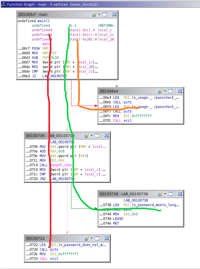
Once we get this compiled and analyzed in Ghidra, we can see the following graph view of main():

‘Blocks’ is one of those intuitive terms, we can see how the graph view automatically breaks down main() into blocks of code. If you look inside each block, you will see that code execution is unidirectional, there are no opportunities inside of a block to take two or more different paths. The code execution is on rails and the train track has no forks. You can see that blocks terminate in this example with conditional jumps (JZ, JNZ), main returning, and function calls to exit.

Edges/Branches/Transitions

‘Edge’ is one of those terms in CS/graph theory that I don’t think is super intuitive and I much prefer ‘Transition’ or ‘Branch’, but essentially this is meant to capture relationships between basic blocks. Looking back at our basic block graph from Ghidra, we can see that a few different relationships exist, that is to say that there are multiple pathways code execution can take depending on a few conditions.

Basic block 001006cf has a relationship with two different blocks: 001006e4 and 00100706. So code execution inside of 001006cf can reach either of the two blocks it has a relationship with depending on a condition. That condition in our case is the JZ operation depending on whether or not the number of command line arguments is 2:

• if the number of arguments is not 2, we branch to block 001006e4 organically by just not taking the conditional jump (JZ)
• if the number of arguments is 2, we branch to block 00100706 by taking the conditional jump

These two possibilities can be referred to as ‘Edges’, so block 01006cf has two edges. You can imagine how this might be important from the perspective of fuzzing. If our fuzzer is only ever exploring one of a basic block’s edges, we are leaving an entire branch untested so it would behoove us to track this type of information.

There’s apparently much more to this concept than I let on here, you can read more on the Wikipedia entry for Control-flow_graph.

Paths

‘Path’ is just the list of basic blocks our program execution traversed. Looking at our example program, there a few different paths as illustrated below with the orange, green and red lines.

Path One: 0x001006cf -> 0x001006e4

Path Two: 0x001006cf -> 0x00100706 -> 0x00100738

Path Three: 0x001006cf -> 0x00100706 -> 0x0000722

Instrumentation

In this blogpost, “Instrumentation” will refer to the process of equipping your fuzzing target with the ability to provide code coverage feedback data. This could mean lots of things. It could be as complex as completely rewriting a compiled binary blob that we have no source code for or as simple as placing a breakpoint on the address of every basic block entry address.

One of the important aspects of instrumentation to keep in mind is the performance penalty incurred by your instrumentation. If your instrumentation provides 50% more useful information than a technique that is 50% less useful but 1000x more performant, you have to consider the tradeoffs. The 50% more data might very well be worth the huge performance penalty, it just depends.

Binary Only

This is a simple one, “Binary Only” refers to targets that we don’t have source code for. So all we have to work with is a binary blob. It can be dynamically linked or static. These types of targets are more prevalent in certain environments, think embedded targets, MacOS, and Windows. There are still binary-only targets on Linux though, they’re just less common.

Even though “binary only” is simple to understand, the implications for gathering code coverage data are far-reaching. A lot of popular code coverage mechanisms rely upon having source code so that the target can be compiled in a certain way that lends itself well to gathering coverage data, for binary-only targets we don’t have the luxury of compiling the target the way that we want. We have to deal with the compiled target the way it is.

Common Strategies

In this section we’ll start looking at common strategies fuzzing tools utilize to gather code coverage data.

Tracking Basic Blocks

One of the most simple ways to gather code coverage is to simply track how many basic blocks are reached by a given input. You can imagine that we are exploring a target program with our inputs and we want to know what code has been reached. Well, we know that given our definition of basic blocks above, if we enter a basic block we will execute all of the code within, so if we just track whether or not a basic block has been reached, we will at least know what paths we have not yet hit and we can go manually inspect them.

This approach isn’t very sophisticated and kind of offers little in the way of high-fidelity coverage data; however, it is extremely simple to implement and works with all kinds of targets. Don’t have source? Throw some breakpoints on it. Don’t have time to write compiler code? Throw some breakpoints on it.

Performance wise, this technique is great. Hitting new coverage will entail hitting a breakpoint, removing the breakpoint and restoring the original contents that were overwritten during instrumentation, saving the input that reached the breakpoint, and continuing on. These events will actually be slow when they occur; however, as you progress through your fuzzing campaign, new coverage becomes increasingly rare. So there is an upfront cost that eventually decreases to near-zero as time goes by.

I’d say that in my limited experience, this type of coverage is typically employed against closed-source targets (binary-only) where our options are limited and this low-tech method works well enough.

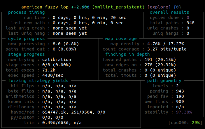
Let’s check out @gamozolabs really fast Basic Block tracking coverage tool called Mesos. You can see that it is aimed at use on Windows where most targets will be binary-only. The neat thing about this tool is its performance. You can see his benchmark results in the README:

Registered    1000000 breakpoints in   0.162230 seconds |  6164072.8 / second
Applied       1000000 breakpoints in   0.321347 seconds |  3111897.0 / second
Cleared       1000000 breakpoints in   0.067024 seconds | 14920028.6 / second
Hit            100000 breakpoints in  10.066440 seconds |     9934.0 / second

One thing to keep in mind is that if you use this way of collecting coverage data, you might limit yourself to the first input that reaches a basic block. Say for instance we have the following code:

// input here is an unsigned char buff
if (input[0x9] < 220)
{
    parsing_routine_1(input);
}

else
{
    parsing_routine_2(input);
}

If our first input to reach this code has a value of 200 inside of input[0x9], then we will progress to the parsing_routine_1 block entry. We will remove our breakpoint at the entry of parsing_routine_1 and we will add the input that reached it to our corpus. But now that we’ve reached our block with an input that had a value of 200, we’re kind of married to that value as we will never hit this breakpoint again with any of the other values that would’ve reached it as well. So we’ll never save an input to the corpus that “solved” this basic block a different way. This can be important. Let’s say parsing_routine_1 then takes the entire input, and reads through the input byte-by-byte for the entirety of the input’s length and does some sort of lengthy parsing at each iteration. And let’s also say there are no subsequent routines that are highly stateful where large inputs vary drastically from smaller inputs in behavior. What if the first input we gave the program that solved this block is 1MB in size? Our fuzzers are kind of married to the large input we saved in the corpus and we were kind of unlucky that shorter input didn’t solve this block first and this could hurt performance.

One way to overcome this problem would be to just simply re-instantiate all of your breakpoints periodically. Say you have been running your fuzzer for 10 billion fuzz-cases and haven’t found any new coverage in 24 hours, you could at that point insert all of your already discovered breakpoints once again and try to solve the blocks in a different way perhaps saving a smaller more performant input that solved the block with a input[0x9] = 20. Really there a million different ways to solve this problem. I believe @gamozolabs addressed this exact issue before on Twitter but I wasn’t able to find the post.

All in all, this is a really effective coverage method especially given the variety of targets it works for and how simple it is to implement.

Tracking Edges and Paths

Tracking edges is very popular because this is the strategy employed by AFL and its children. This is the approach where we not only care about what basic blocks are being hit but also, what relationships are being explored between basic blocks.

The AFL++ stats output has references to both paths and edges and implicitly ‘counters’. I’m not 100% sure but I believe their definition of a ‘path’ matches up to ours above. I think they are saying that a ‘path’ is the same as a testcase in their documentation.

I won’t get too in-depth here analyzing how AFL and its children (really AFL++ is quite different than AFL) collect and analyze coverage for a simple reason: it’s for big brain people and I don’t understand much of it. If you’re interested in a more detailed breakdown, head on over to their docs and have a blast.

To track edges, AFL uses tuples of the block addresses involved in the relationship. So in our example program, if we went from block 0x001006cf to block 0x001006e4 because we didn’t provide the correct number of command line arguments, this tuple (0x001006cf , 0x001006e4) would be added to a coverage map AFL++ uses to track unique paths. So let’s track the tuples we would register if we traversed an entire path in our program:

0x001006cf -> 0x00100706 -> 0x00100722

If we take the above path, we can formulate two tuples of coverage data: (0x001006cf, 0x00100706) and (0x00100706, 0x00100722). These can be looked up in AFL’s coverage data to see if these relationships have been explored before.

Not only does AFL track these relationships, it also tracks frequency. So for instance, it is aware of how often each particular edge is reached and explored.

This kind of coverage data is way more complex than merely tracking basic blocks reached; however, getting this level of detail is also not nearly as straightforward.

In the most common case, AFL gets this data by using compile-time instrumentation on the target. You can compile your target, that you have source code for, using the AFL compiler which will emit compiled code with the instrumentation embedded in the target. This is extremely nifty. But it requires access to source code which isn’t always possible.

AFL has an answer for binary-only targets as well and leverages the powerful QEMU emulator to gather similarly detailed coverage data. Emulators have relatively free access to this type of data since they have to take the target instructions and either interpret them (which means simulate their execution) or JIT (just-in-time) compile the blocks into native code and execute them natively. In the case of QEMU here, blocks are JIT’d into native code and stored in a cache so that it could be easily used again by subsequent executions. So when QEMU comes upon a basic block, it can check whether or not this block has been compiled or not already and act accordingly. AFL utilizes this process to track what blocks are being executed and gets very similar data to what it gathers with compile time instrumentation.

I don’t understand all of the nuance here, but a great blogpost to read on the subject is: @abiondo’s post explaining an optimization they made to AFL QEMU mode in 2018. In a grossly short (hopefully not too inaccurate) summary, QEMU would pre-compute what are called direct jumps and compile those blocks into a single block essentially (via keeping execution in natively compiled blocks) as a way to speed things up. Take this toy example for instance:

ADD RAX, 0x8
JMP LAB_0x00100738

Here we have a pre-computable destination to our jump. We know the relative offset to LAB_0x00100738 from our current address (absolute value of current_addr - LAB_0x00100738), so in an emulator we could just take that jump and replace the destination to the compiled block of LAB_0x00100738 and no calculations would need to take place during each execution (only the initial one to calculate the relative offset). This would allow the emulator to progress with native execution without going back into what I would call a ‘simulation-mode’ where it has to calculate the address before jumping to it each time its executed. This is called “block-chaining” in QEMU. Well you can imagine that if this occurs, that huge block of natively executed code (that is really two blocks) is completely opaque to AFL as it’s unaware that two blocks are contained and so it cannot log the edge that was taken. So as a work around, AFL would patch QEMU to no longer do this block-chaining and keep every block isolated so that edges could be tracked. This would mean that at the end of every block, direct jump or not, QEMU would go back into that ‘simulation-mode’ which would incur a performance penalty.

Definitely read through @abiondo’s blogpost though, it’s much more informative.

If you’re wondering what an indirect jump would be, it would be something where the jump location is only known at execution time, something that could look like this in a toy example:

ADD RAX, 0x8
JMP RAX

The only issue with using QEMU to gather our coverage data is it is relatively slow compared to purely native execution. This slowdown can be worth it obviously as the amount of data you get is substantial and sometimes with binary-only targets there are no other alternatives.

Compare Coverage/Compare Shattering

Instead of merely tracking an input or test’s progress through a program’s blocks/edges, compare coverage seeks to understand how much progress our test is making in the program’s comparisons. Comparisons can be done different ways but a common one already exists in our example password program. In the 001006cf block, we have a CMP operation being performed here:

CMP dword ptr [RBP + local_1c], 0x2

A dword is a 4 byte value (32 bits) and this operation is taking our argc value in our program and comparing it with 0x2 to check how many command line arguments were provided. So our two comparison operands are whatever is on the stack at the offset RBP + local_1c and 0x2. If these operands are equal, the Zero Flag will be set and we can utilize a conditional jump with JZ to move accordingly in the program.

But the problem, as it relates to fuzzing, is that this comparison is rather binary. It either sets the Zero Flag or it does not, there is no nuance. We cannot tell how close we came to passing the comparison, to setting the Zero Flag.

So for example, let’s say we were doing a comparison with 0xdeadbeef instead of 0x2. In that case, if we were to submit 0xdeadbebe for the other operand, we’d be much closer to satisfying the JZ condition that we would be if we submitted 0x0.

At a high-level, compare coverage breaks this comparison down into chunks so that progress through the comparison can be tracked with more much granularity than a binary PASS/FAIL. So using compare coverage, this comparison might instead be rewritten as follows:

BEFORE:

Does 0xdeadbebe == 0xdeadbeef ?

AFTER:

Does 0xde == 0xde ? If so, log that we’ve matched the first byte, and

does 0xad == 0xad ? If so, log that we’ve matched the second byte, and

does 0xbe == 0xbe ? If so, log that we’ve matched the third byte, and

does 0xbe == 0xef ? If so, log that we’ve matched both operands completely.

In our AFTER rewrite, instead of getting a binary PASS/FAIL, we instead see that we progressed 75% of the way through the comparison matching 3 out of 4 bytes. Now we know that we can save this input and mutate it further hoping that we can pass the final byte comparison with a correct mutation.

We also aren’t restricted to only breaking down each comparison to bytes, we could instead compare the two operands at the bit-level. For instance we could’ve also compared them as follows:

1101 1110 1010 1101 1011 1110 1110 1111 vs

1101 1110 1010 1101 1011 1110 1011 1110

This could be broken down into 32 separate comparisons instead of our 4, giving us even more fidelity and progress tracking (probably at the expense of performance in practice).

Here we took a 4 byte comparison and broke it down into 4 separate single-byte comparisons. This is also known as “Compare Shattering”. In spirit, it’s very similar to compare coverage. It’s all about breaking down large comparisons into smaller chunks so that progress can be tracked with more fidelity.

Some fuzzers take all compare operands, like 0xdeadbeef in this example, and add them to a sort of magic values dictionary that the fuzzer will randomly insert it into its inputs hoping to pass the comparison in the future.

You can imagine a scenario where a program checks a large value before branching to a complex routine that needs to be explored. Passing these checks is extremely difficult with just basic coverage and would require a lot of human interaction. One could examine a colored graph in IDA that displayed reached blocks and try to manually figure out what was preventing the fuzzer from reaching unreached blocks and determine that a large 32 byte comparison was being failed. One could then adjust their fuzzer to account for this comparison by means of a dictionary or whatever, but this process is all very manual.

There are some really interesting/highly technical means to do this type of thing to both targets with source and binary-only targets!

AFL++ features an LLVM mode where you can utilize what they call “laf-intel instrumentation” which is described here and originally written about here. Straight from laf-intel’s blogpost, we can see their example looks extremely similar to the thought experiment we already went through where they have this source code:

if (input == 0xabad1dea) {
  /* terribly buggy code */
} else {
  /* secure code */
}

And this code snippet is ‘de-optimized’ into several smaller comparisons that the fuzzer can measure its progress through:

if (input >> 24 == 0xab){
  if ((input & 0xff0000) >> 16 == 0xad) {
    if ((input & 0xff00) >> 8 == 0x1d) {
      if ((input & 0xff) == 0xea) {
        /* terrible code */
        goto end;
      }
    }
  }
}

/* good code */

end:

This de-optimized code can be emitted when one opts to specify certain environment variables and utilizes afl-clang-fast to compile the target.

This is super clever and can really take tons of manual effort out of fuzzing.

But what are we to do when we don’t have access to source code and our binary-only target is possibly full of large comparisons?

Luckily, there are open-source solutions to this problem as well. Let’s look at one called “TinyInst” by @ifsecure and friends. I can’t get deep into how this tool works technically because I’ve never used it but the README is pretty descriptive!

As we can see, it is aimed at MacOS and Windows targets in-keeping with its purpose of instrumenting binary only targets. TinyInst gets us coverage by instrumenting select routines via debugger to change the execution permissions so that any execution (not read or write as these permissions are maintained) access to our instrumented code results in a fault which is then handled by the TinyInst debugger where code execution is redirected a re-written instrumented routine/module. So TinyInst blocks all execution of the original module and instead, redirects all that execution to a rewritten module that is inserted into the program. You can see how powerful this can be as it can allow for the breaking down of large comparisons into much smaller ones in a manner very similar to the laf-intel method but for a target that is already compiled. Look at this cool gif showing compare coverage in action from @ifsecure: [https://twitter.com/ifsecure/status/1298341219614031873?s=20]. You can see that he has a program that checks for an 8 byte value, and his fuzzer makes incremental progress through it until it has solved the comparison.

There are some other tools out there that work similarly in theory to TinyInst as well that are definitely worth looking at and they are also mentioned in the README, tools like: DynamoRIO and PIN.

It should also be mentioned that AFL++ also has the ability to do compare coverage tracking even in QEMU mode.

Bonus Land: Using Hardware to Get Coverage Data

That pretty much wraps up the very basics of what type of data we’re interested in, why, and how we might be able to extract it. One type of data extraction method that didn’t come up yet that is particularly helpful for binary-only targets is utilizing your actual hardware to get coverage data.

While it’s not really a ‘strategy’ as the others were, it enables the execution of the strategies mentioned above and wasn’t mentioned yet. We won’t get too deep here. Nowadays, CPUs come chock-full of all kinds of utilities that are aimed at high-fidelity performance profiling. These types of utilities can also be wrangled into giving us coverage data.

Intel-PT is a utility offered by newer Intel CPUs that allows you to extract information about the software you’re running such as control-flow. Each hardware thread has the ability to store data about the application it is executing. The big hang up with using processor trace is that decoding the trace data that is collected has always been painfully slow and cumbersome to work with. Recently however, @is_eqv and @ms_s3c were able to create a very performant library called libxdc which can be used to decode Intel-PT trace data performantly. The graph included in their README is very cool, you can see how much faster it is than the other hardware-sourced coverage guided fuzzing tools while also collecting the highest-fidelity coverage data, what they call “Full Edge Coverage”. Getting your coverage data straight from the CPU seems ideal haha. So for them to be able to engineer a library that gives you what is essentially perfect coverage, and by the way, doesn’t require source code, seems like a substantial accomplishment. I personally don’t have the engineering chops to deal with this type of coverage at the moment, but one day. A lot of popular fuzzers can utilize Intel-PT right out of the box, fuzzers like: AFL++, honggfuzz, and WinAFL.

There are many other such utilities but they are beyond the scope of this introductory blogpost.

Conclusion

In this post we went over some of the building-block terminology used in the space, some very common fundamental strategies that are employed to get meaningful coverage data, and also some of the tooling that is used to extract the data (and in some cases what fuzzing frameworks use what tooling). It should be mentioned that the popular fuzzing frameworks like AFL++ and honggfuzz go through great lengths to make their frameworks as flexible as possible and work with a wide breadth of targets. They often give you tons of flexibility to employ the coverage data extraction method that’s best suited to your situation. Hopefully this was somewhat helpful to begin to understand some of the problems associated with code coverage as it relates to fuzzing.